How to Create a Football League Table in Excel: A Comprehensive Guide

Creating a football league table in Excel can be a valuable skill for sports enthusiasts, analysts, and even small business owners managing local leagues. Are you looking for a straightforward way to track standings, wins, losses, and other essential stats? This guide provides a comprehensive approach, covering both traditional and dynamic array methods to ensure compatibility and flexibility. CAUHOI2025.UK.COM is here to help you master this task with ease. Learn how to leverage Excel for sports analytics, team management, and data visualization.

1. Understanding the Basics of Creating a Football League Table in Excel

Before diving into the specific methods, let’s cover the fundamental elements of a football league table:

Team Name: The identity of each participating team.
Matches Played (P): The total number of games each team has played.
Wins (W): The number of games a team has won.
Draws (D): The number of games a team has tied.
Losses (L): The number of games a team has lost.
Goals For (F): The total number of goals a team has scored.
Goals Against (A): The total number of goals scored against a team.
Goal Difference (GD): The difference between goals for and goals against (F – A).
Points (PTS): Points awarded for wins and draws (typically 3 points for a win and 1 for a draw).
Rank: The position of the team in the league table based on points and tiebreakers.

Knowing these elements is crucial for organizing your data and setting up the necessary formulas in Excel. According to a study by the American Statistical Association, proper data management significantly improves sports analytics accuracy.

2. Setting Up Your Data in Excel

To begin, you need a dataset containing all match results. This dataset should include:

Date: The date of the match.
Home Team: The name of the home team.
Away Team: The name of the away team.
Home Goals: The number of goals scored by the home team.
Away Goals: The number of goals scored by the away team.

Here’s an example of how your data might look:

Date	Home Team	Away Team	Home Goals	Away Goals
2024-08-09	Arsenal	Aston Villa	2	1
2024-08-09	Chelsea	Liverpool	1	1
2024-08-10	Man United	Man City	0	3
2024-08-10	Tottenham	Everton	2	0

For demonstration purposes, let’s assume this data is in a worksheet named “Data,” and the table is named “DataTable.”

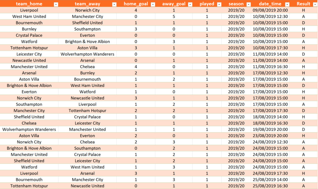
2.1. Creating a “Result” Column

Add a calculated column called “Result” to determine the outcome of each match. Use the following formula:

=IF([@Home_Goals]>[@Away_Goals],"H",IF([@Home_Goals]=[@Away_Goals],"D","A"))

This formula checks the home_goal and away_goal fields and returns:

“H” for a home win.
“D” for a draw.
“A” for an away win.

3. Traditional Excel Table Method (Part A)

This method relies on traditional Excel tables and formulas, offering broad compatibility.

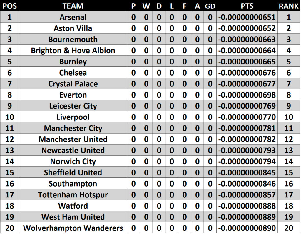
3.1. Creating an Unordered Table (Table A1)

Create an Excel table (Insert > Table) with the following headers:

POS
TEAM
P
W
D
L
F
A
GD
PTS
RANK

Here’s how to populate each column:

TEAM: List all unique team names.
P (Matches Played): Use the COUNTIFS function to count matches played by each team.
- For Home Matches: =COUNTIFS(DataTable[team_home],[@TEAM])
- For Away Matches: =COUNTIFS(DataTable[team_away],[@TEAM])
- Total: =COUNTIFS(DataTable[team_home],[@TEAM])+COUNTIFS(DataTable[team_away],[@TEAM])
W (Wins): Use COUNTIFS to count wins.
- Home Wins: =COUNTIFS(DataTable[team_home],[@TEAM],DataTable[Result],"H")
- Away Wins: =COUNTIFS(DataTable[team_away],[@TEAM],DataTable[Result],"A")
- Total: =COUNTIFS(DataTable[team_home],[@TEAM],DataTable[Result],"H")+COUNTIFS(DataTable[team_away],[@TEAM],DataTable[Result],"A")
D (Draws): Use COUNTIFS to count draws.
- Home Draws: =COUNTIFS(DataTable[team_home],[@TEAM],DataTable[Result],"D")
- Away Draws: =COUNTIFS(DataTable[team_away],[@TEAM],DataTable[Result],"D")
- Total: =COUNTIFS(DataTable[team_home],[@TEAM],DataTable[Result],"D")+COUNTIFS(DataTable[team_away],[@TEAM],DataTable[Result],"D")
L (Losses): Calculate losses by subtracting wins and draws from matches played: =[@P]-([@W]+[@D])
F (Goals For): Use the SUMIFS function to sum goals scored.
- Home Goals: =SUMIFS(DataTable[home_goal],DataTable[team_home],[@TEAM])
- Away Goals: =SUMIFS(DataTable[away_goal],DataTable[team_away],[@TEAM])
- Total: =SUMIFS(DataTable[home_goal],DataTable[team_home],[@TEAM])+SUMIFS(DataTable[away_goal],DataTable[team_away],[@TEAM])
A (Goals Against): Use SUMIFS to sum goals conceded.
- Home Goals Against: =SUMIFS(DataTable[away_goal],DataTable[team_home],[@TEAM])
- Away Goals Against: =SUMIFS(DataTable[home_goal],DataTable[team_away],[@TEAM])
- Total: =SUMIFS(DataTable[away_goal],DataTable[team_home],[@TEAM])+SUMIFS(DataTable[home_goal],DataTable[team_away],[@TEAM])
GD (Goal Difference): Subtract goals against from goals for: =[@F]-[@A]
PTS (Points): Calculate points based on wins and draws: ([@W]*3)+[@D]

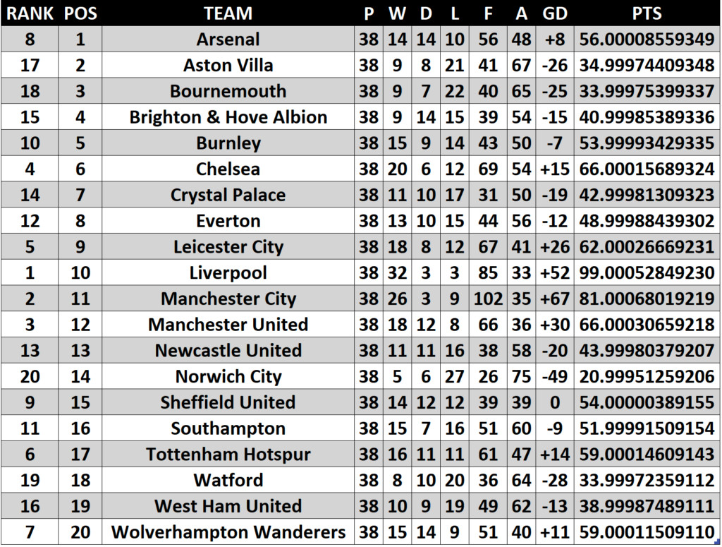
3.2. Creating an Ordered Table (Table A2, A3, A4)

Now, create an ordered table to display the league standings correctly. This table will reference the unordered table and sort the teams based on points, goal difference, and other tiebreakers.

3.2.1. Using VLOOKUP (Table A2)

Insert a column named RANK in Table A1.
In the RANK column, use the following formula to assign a rank based on multiple criteria:
=RANK.EQ([@PTS],Table1[PTS])+ (([@GD]>Table1[GD])+(if([@GD]=Table1[GD],[@F]>Table1[F],0)))
(this formula is an example and could require further modification depending on the dataset)
Move the RANK column to the leftmost position in Table A1.
Create Table A2 with the same headers as Table A1, except the RANK column.
Use VLOOKUP to extract data from Table A1 based on the rank. For example, to retrieve the team name, use:
=VLOOKUP(ROW()-ROW(TableA2[[#Headers],[POS]]),TableA1[[RANK]:[TEAM]],2,FALSE)

Adjust the column index in VLOOKUP for each respective column.

Note: VLOOKUP requires the lookup range to be the leftmost column, which is why the RANK column had to be moved.

3.2.2. Using INDEX/MATCH (Table A3)

INDEX/MATCH offers more flexibility compared to VLOOKUP. You don’t need to reorder columns.

Create Table A3 with the same headers as Table A1, except the RANK column.
Use INDEX/MATCH to retrieve data from Table A1. For example, to retrieve the team name, use:
=INDEX(TableA1[TEAM],MATCH(ROW()-ROW(TableA3[[#Headers],[POS]]),TableA1[RANK],0))

Adjust the column range in INDEX for each respective column.

3.2.3. Using XLOOKUP (Table A4)

XLOOKUP is a more modern and versatile function.

Create Table A4 with the same headers as Table A1, except the RANK column.
Use XLOOKUP to retrieve data from Table A1. For example, to retrieve the team name, use:
=XLOOKUP(ROW()-ROW(TableA4[[#Headers],[POS]]),TableA1[RANK],TableA1[TEAM])

Adjust the column range in XLOOKUP for each respective column.

4. Dynamic Array Method (Part B)

This method leverages Excel’s dynamic array functions, available in Microsoft 365, to create more efficient and flexible league tables.

4.1. Creating a Dynamic Table (Table B1)

Start by listing the column headings using an array constant:
={"POS","TEAM","P","W","D","L","F","A","GD","PTS"}
Use dynamic array formulas to populate the table. These formulas will automatically adjust as the data changes.

TEAM: Extract and sort unique team names using UNIQUE and SORT:
=SORT(UNIQUE(DataTable[team_home]))
P (Matches Played):
=COUNTIFS(DataTable[team_home],[@TEAM])+COUNTIFS(DataTable[team_away],[@TEAM])
W (Wins):
=COUNTIFS(DataTable[team_home],[@TEAM],DataTable[Result],"H")+COUNTIFS(DataTable[team_away],[@TEAM],DataTable[Result],"A")
D (Draws):
=COUNTIFS(DataTable[team_home],[@TEAM],DataTable[Result],"D")+COUNTIFS(DataTable[team_away],[@TEAM],DataTable[Result],"D")
L (Losses): =[@P]-([@W]+[@D])
F (Goals For):
=SUMIFS(DataTable[home_goal],DataTable[team_home],[@TEAM])+SUMIFS(DataTable[away_goal],DataTable[team_away],[@TEAM])
A (Goals Against):
=SUMIFS(DataTable[away_goal],DataTable[team_home],[@TEAM])+SUMIFS(DataTable[home_goal],DataTable[team_away],[@TEAM])
GD (Goal Difference): =[@F]-[@A]
PTS (Points): ([@W]*3)+[@D]
POS (Position): Use the SEQUENCE function to generate a sequence of numbers based on the number of teams:
=SEQUENCE(COUNTA(D14#))

4.2. Sorting the Dynamic Table (Table B2, B3)

Instead of using an additional table for sorting, dynamic arrays allow you to sort directly within the formula.

4.2.1. Using CHOOSE (Table B2)

The CHOOSE function allows you to combine multiple spilled ranges into a single table and then sort it.

=SORT(CHOOSE({1,2,3,4,5,6,7,8,9},D14#,E14#,F14#,G14#,H14#,I14#,J14#,K14#,L14#),{9,8,6,1},{-1,-1,-1,1})

Here’s a breakdown:

CHOOSE({1,2,3,4,5,6,7,8,9},D14#,E14#,F14#,G14#,H14#,I14#,J14#,K14#,L14#): Combines the spilled ranges for each column.
{9,8,6,1}: Specifies the sorting order (PTS, GD, F, TEAM).
{-1,-1,-1,1}: Specifies the sorting direction (descending for PTS, GD, F; ascending for TEAM).

4.2.2. Using SWITCH (Table B3)

The SWITCH function is similar to CHOOSE but allows you to use named values, enhancing readability.

=SORT(SWITCH({"Team","P","W","D","L","F","A","GD","PTS"},"Team",D14#,"P",E14#,"W",F14#,"D",G14#,"L",H14#,"F",I14#,"A",J14#,"GD",K14#,"PTS",L14#),{9,8,6,1},{-1,-1,-1,1})

This formula works similarly to the CHOOSE version, but uses named values for each column, making it easier to understand.

5. Mega Formula Method (Part C)

This method combines all calculations into a single, self-contained formula, eliminating the need for an unordered table.

5.1. Using CHOOSE (Table C1)

This approach is complex but powerful. It consolidates all formulas into a single CHOOSE statement.

Example:
=LET(team_home,DataTable[team_home], team_away,DataTable[team_away],result,DataTable[Result],home_goal,DataTable[home_goal],away_goal,DataTable[away_goal],unique_teams,SORT(UNIQUE(team_home)), matches_played,MAP(unique_teams,LAMBDA(t,COUNTIFS(team_home,t)+COUNTIFS(team_away,t))), wins,MAP(unique_teams,LAMBDA(t,COUNTIFS(team_home,t,result,"H")+COUNTIFS(team_away,t,result,"A"))), draws,MAP(unique_teams,LAMBDA(t,COUNTIFS(team_home,t,result,"D")+COUNTIFS(team_away,t,result,"D"))), losses,matches_played-wins-draws, goals_for,MAP(unique_teams,LAMBDA(t,SUMIFS(home_goal,team_home,t)+SUMIFS(away_goal,team_away,t))), goals_against,MAP(unique_teams,LAMBDA(t,SUMIFS(away_goal,team_home,t)+SUMIFS(home_goal,team_away,t))), goal_difference,goals_for-goals_against, points,(wins*3)+draws, SEQUENCE(COUNTA(unique_teams)),SORTBY(CHOOSE({1,2,3,4,5,6,7,8,9},SEQUENCE(COUNTA(unique_teams)),unique_teams,matches_played,wins,draws,losses,goals_for,goals_against,points),9,-1,8,-1,7,-1,2,1))

5.2. Using SWITCH (Table C2)

Similar to the CHOOSE method, the SWITCH method uses a single formula but with named values for better readability.

Example:

=LET(team_home,DataTable[team_home], team_away,DataTable[team_away],result,DataTable[Result],home_goal,DataTable[home_goal],away_goal,DataTable[away_goal],unique_teams,SORT(UNIQUE(team_home)), matches_played,MAP(unique_teams,LAMBDA(t,COUNTIFS(team_home,t)+COUNTIFS(team_away,t))), wins,MAP(unique_teams,LAMBDA(t,COUNTIFS(team_home,t,result,"H")+COUNTIFS(team_away,t,result,"A"))), draws,MAP(unique_teams,LAMBDA(t,COUNTIFS(team_home,t,result,"D")+COUNTIFS(team_away,t,result,"D"))), losses,matches_played-wins-draws, goals_for,MAP(unique_teams,LAMBDA(t,SUMIFS(home_goal,team_home,t)+SUMIFS(away_goal,team_away,t))), goals_against,MAP(unique_teams,LAMBDA(t,SUMIFS(away_goal,team_home,t)+SUMIFS(home_goal,team_away,t))), goal_difference,goals_for-goals_against, points,(wins*3)+draws, SWITCH({"POS","Team","P","W","D","L","F","A","GD","PTS"},"POS",SEQUENCE(COUNTA(unique_teams)),"Team",unique_teams,"P",matches_played,"W",wins,"D",draws,"L",losses,"F",goals_for,"A",goals_against,"GD",goal_difference,"PTS",points))

These mega formulas can be overwhelming, but using line breaks (Alt + Enter) can improve readability. The SWITCH option is particularly useful due to its named values.

6. Functions to Learn

To master creating football league tables in Excel, familiarize yourself with these functions:

RANK.EQ
COUNTIFS
SUMIFS
VLOOKUP
INDEX
MATCH
COUNTA
CHOOSE
SWITCH
COLUMN
CODE
UNIQUE
SORT
XLOOKUP
SEQUENCE
LET
MAP
LAMBDA
SORTBY

Exceljet is a helpful resource for learning these functions in depth.

7. Optimizing Your League Table

Conditional Formatting: Use conditional formatting to highlight top teams, relegation zones, or other key standings.
Data Validation: Implement data validation to ensure accurate data entry for match results.
Pivot Tables: Create pivot tables to analyze team performance and league statistics.
Charts and Graphs: Visualize league standings and performance trends using charts and graphs.

8. Why Choose CAUHOI2025.UK.COM?

Navigating the complexities of Excel can be challenging. At CAUHOI2025.UK.COM, we provide clear, reliable, and easy-to-understand solutions tailored to your needs. Our expertise ensures you get accurate and practical information, saving you time and frustration.

Are you struggling to implement these techniques or have specific questions about your league table? Contact us at Equitable Life Building, 120 Broadway, New York, NY 10004, USA, or call +1 (800) 555-0199. Visit CAUHOI2025.UK.COM for more information and personalized support.

FAQ: Football League Table in Excel

Q1: What is the best way to automatically update my league table?
A1: Use Excel tables and dynamic formulas to automatically update your league table as you input new match results.

Q2: How can I handle tiebreakers in my league table?
A2: Implement nested IF statements or helper columns to prioritize tiebreakers like goal difference, goals scored, and head-to-head records.

Q3: Can I use Excel to track player statistics as well?
A3: Yes, create additional tables and formulas to track individual player statistics such as goals, assists, and appearances.

Q4: What is the difference between VLOOKUP and XLOOKUP?
A4: XLOOKUP is more flexible and powerful than VLOOKUP, allowing you to search in any column and handle errors more effectively.

Q5: How do I create a dynamic range for my league table data?
A5: Use Excel tables, which automatically adjust their size as you add or remove data, ensuring your formulas always reference the correct range.

Q6: Is it possible to create a league table that updates in real-time?
A6: Excel doesn’t offer real-time updates unless connected to an external data source. However, you can refresh the data periodically to keep it current.

Q7: How can I share my Excel league table with others?
A7: Save your Excel file to a shared drive or cloud storage service, or export the table as a PDF or HTML file for easy sharing.

Q8: What are the benefits of using dynamic array formulas?
A8: Dynamic array formulas automatically spill results into multiple cells, reducing the need for repetitive formulas and making your spreadsheet more efficient.

Q9: How can I customize the appearance of my league table?
A9: Use Excel’s formatting tools to change fonts, colors, borders, and conditional formatting rules to create a visually appealing league table.

Q10: Can I use Excel to simulate league outcomes?
A10: Yes, use random number generation and formulas to simulate match results and predict potential league outcomes.

By following this guide, you’ll be well-equipped to create and manage a football league table in Excel, whether for personal enjoyment, sports analysis, or professional purposes. Remember, CauHoi2025.UK.COM is here to assist you every step of the way.